One of the best ways you can represent numerical data is by using bar graphs. For instance, if you want to represent a trend that has been growing over time, using a bar graph will make it much easier for the audience to understand than leaving the numerical data in tables. Fortunately, it is very easy to create bar graphs in excel if you know the exact procedures to use.
In this guide, I will take you through the step-by-step procedure for creating bar graphs in excel. I will be using Excel 2019, but the procedure is pretty similar for Excel 2013, 2016, and 2021.
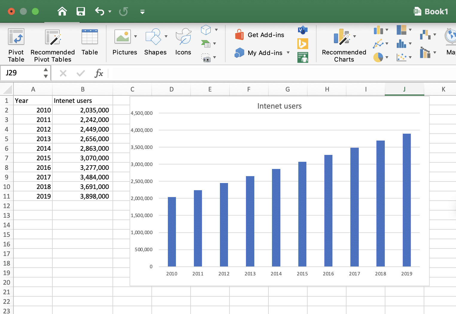
Here’s the chart we will build:
Step #1: Open your Excel 365 sheet
Open the excel application and retrieve the sheet containing the data you intend to represent with the bar graph.
Step #2: Highlight your data range
Select the columns containing the data that you want to represent in your bar graph. In my case, I selected columns A(year) and B (number of internet users). If the columns of the data you want to turn into a bar graph are not next to each other, here is how you select them. Select the first column, press Ctrl for Windows or Command for macOS, and then select the second column.
Step #3: Insert your bar plot in Excel
While your columns are still highlighted, hit Insert (the second menu bar from the left). There will be a wide range of bar graph options that you can choose from. After highlighting the data you want to plot, Excel will give you a couple of bar graph suggestions under Recommended charts. Most of the time, you will find one or two options that will best represent the data you have selected. In this case, With the example above, I chose the clustered column option that was under Recommended charts.
Step #4: Further customization
You can customize your bar graph to give it your desired look, for example insert callouts and labels to your chart. Simply right-click at any point within the chart to view all the available customization options.
FAQ
How to change the order of the bars in my Excel chart?
You can reorder the bar chart using the following process:
- Open Excel.
- In your spreadsheet, highlight any of the cells of your dataset.
- Then go to the Data tab.
- Use the Sort button to arrange your data according to your preferences.
- Your chart bars will be rearranged automatically.
- Save your spreadsheet.
How to create a trendline for your bar chart?
You can easily create a regression line for your bar / scatter / combo chart. Look at this tutorial for more details.