You built your VLOOKUP formula, pressed Enter, and got #N/A staring back at you. The formula looks right, the data is clearly there in the other sheet, but Excel refuses to return a match. This almost always comes down to invisible formatting differences between your lookup value and your table data — not a broken formula.
Three causes account for the vast majority of VLOOKUP failures, and each one has a specific fix that takes under a minute.
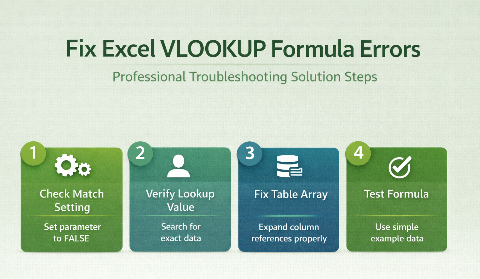
Fix the most common VLOOKUP errors
Check the match type argument
Click on your VLOOKUP formula and look at the last argument — if it says TRUE or is missing entirely, that is your problem. Change it to FALSE so the formula reads something like =VLOOKUP(A2,Sheet2!B:E,3,FALSE). The TRUE setting tells Excel to find an approximate match using sorted data, and when your table is not sorted in strict ascending order, it returns garbage values or #N/A without any warning whatsoever. FALSE forces an exact match, which is what you want in nearly every real-world scenario where you are looking up specific product codes, employee IDs, or category names.
Strip hidden spaces from cells
The value “Apple” and “Apple ” look identical on screen, but VLOOKUP treats them as completely different entries because that trailing space changes the text comparison result. Select your lookup column, press Ctrl+H to open Find and Replace, put a single space in the Find what field, leave Replace with empty, and click Replace All. Do the same for the first column of your table array. This one step resolves a surprising number of lookup failures, especially with data pasted from web pages, exported from CRM systems, or imported from databases where trailing whitespace sneaks in during the export process without anyone noticing.
Convert text numbers to real numbers
A cell displaying 1234 might store the value as text “1234” internally, and VLOOKUP will not match text against a number — they are fundamentally different data types in Excel’s comparison engine.
- Look for the small green triangle in the top-left corner of suspect cells — that is Excel warning you the content is stored as text rather than as a numeric value.
- Select those cells, click the warning icon, and choose Convert to Number.
- If you are dealing with an entire column of numbers stored as text, the Data >> Text to Columns wizard with default Delimited settings forces a bulk conversion that fixes every cell in the selection at once.
Verify your table array references
Confirm the lookup column position
VLOOKUP searches only the first column of your table array, so if your lookup value lives in column C but your table array starts at column B, the formula searches column B instead — and naturally finds nothing because it is looking in the wrong place entirely. Adjust your table array range so it starts at the column containing the values you want to match against. The column index number in your third argument counts from that starting column: if your range is B:E, then B is 1, C is 2, D is 3, and E is 4. Getting this count wrong is one of the most common mistakes, especially in workbooks where people insert or delete columns after writing the formula.
Lock references with absolute addresses
When you copy a VLOOKUP formula down a column, relative references shift with each row — your table array drifts and the formula breaks silently, returning wrong results or errors that seem random. Switch to absolute references like $B$2:$E$100 by pressing F4 after selecting the range in your formula. Named ranges work even better for long-term maintainability: select your table, press Ctrl+Shift+F3, give it a name like LookupTable, then rewrite your formula as =VLOOKUP(A2,LookupTable,3,FALSE). The formula becomes readable and completely immune to copy-paste reference drift.
When the formula still returns errors
Step through with Evaluate Formula
Open the Formulas tab, click Evaluate Formula in the Formula Auditing group, and step through each part of your VLOOKUP one piece at a time. Excel shows you exactly where the evaluation fails — whether it cannot find the lookup value, whether the column index is out of range, or whether a data type mismatch is causing the rejection. This built-in debugger saves far more time than staring at the formula bar trying to spot the issue visually, and it catches problems that are completely invisible in the cell display.
Wrap errors with IFERROR
Once you have fixed the root cause, wrap your formula in IFERROR for cleaner output: =IFERROR(VLOOKUP(A2,B:E,3,FALSE),”Not Found”). This replaces ugly #N/A errors with whatever text you choose, making reports and dashboards presentable even when some lookups legitimately have no match. Keep in mind that IFERROR masks all error types rather than solving them — use it for the final presentation layer, not as a substitute for actual troubleshooting, because it will hide genuine formula problems along with expected mismatches.
Switch to INDEX MATCH instead
If your lookup needs to search right-to-left or pull from multiple columns dynamically, VLOOKUP simply cannot do it — it only searches the leftmost column of the table array by design. The formula =INDEX(C:C,MATCH(A2,B:B,0)) does the same job without the first-column restriction and gives clearer error messages when something goes wrong. You can also let Copilot handle complex lookups if you are on Microsoft 365 and want to describe what you need in plain language rather than building formula syntax manually.
Top questions about Excel VLOOKUP
Why does VLOOKUP return #N/A when the value exists?
The value exists visually but not technically. Trailing spaces, text-vs-number mismatches, or non-printable characters copied from external sources make two cells look identical while Excel sees them as different. Use TRIM and CLEAN on both your lookup value and table data to strip hidden differences.
What causes VLOOKUP to return the wrong value?
Using TRUE or omitting the last argument defaults to approximate match mode, which requires your first column sorted in ascending order. If the data is unsorted, Excel picks an incorrect row without warning. Switch the last argument to FALSE for exact matching in virtually all cases.
Should I use XLOOKUP instead of VLOOKUP?
If you have Excel 365 or Excel 2021, yes. XLOOKUP searches any direction, defaults to exact match, handles errors natively with its if_not_found argument, and does not need a column index number. It replaces both VLOOKUP and INDEX/MATCH in most situations.
Start with the match type and hidden spaces — those two fixes clear up the majority of broken VLOOKUPs before you ever need the advanced troubleshooting.